Phonon Calculation

This script will show how to use mdapy to calculate phonon dispersion.

One should install Phonopy by one of the following ways:

• pip install phonopy

• conda install -c conda-forge phonopy

# import necessary package

import mdapy as mp
import numpy as np
import matplotlib.pyplot as plt
mp.init()

[Taichi] version 1.7.1, llvm 15.0.1, commit 0f143b2f, win, python 3.10.14
[Taichi] Starting on arch=x64

print('mdapy version is :', mp.__version__)

mdapy version is : 0.10.9

We use graphene as an example.

# Build a graphene

lat = mp.LatticeMaker(1.42, 'GRA', 1, 1, 1)
lat.compute()

# Add a vacuum layer with 0.2 nm along z direction.
lat.box[2, 2] += 20

# Generate a system

system = mp.System(pos=lat.pos, box=lat.box)

The key step in calculating phonon is obtaining force set from finite displacements. So we need to provide a potential to compute the atomic forces. In mdapy, we originally support NEP and eam/alloy potential. Besides, we also provide a interface to call lammps to computer force, where one need to install lammps-python interface. Further more, user can define a custom potential for whatever you like, and we will discuss latter.

NEP potential

This NEP potential is downloaded from here.

potential = mp.NEP('../../../example/C_2024_NEP4.txt')

potential.info

{'version': 4,
 'zbl': False,
 'radial_cutoff': 7.0,
 'angular_cutoff': 4.0,
 'n_max_radial': 12,
 'n_max_angular': 8,
 'basis_size_radial': 16,
 'basis_size_angular': 12,
 'l_max_3body': 4,
 'num_node': 67,
 'num_para': 7239,
 'element_list': ['C']}

To plot band structure, one need also provide the band path and labels.

One can obtain those by seekpath online.

# For graphene
path = '0.0 0.0 0.0 0.3333333333 0.3333333333 0.0 0.5 0.0 0.0 0.0 0.0 0.0'
labels = '$\Gamma$ K M $\Gamma$'

# Do computation
system.cal_phono_dispersion(path, labels, potential, elements_list=['C'])

Warning: Point group symmetries of supercell and primitivecell are different.

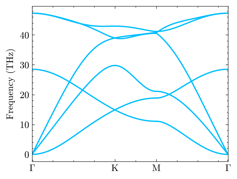
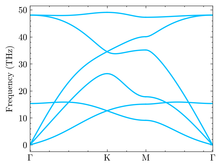
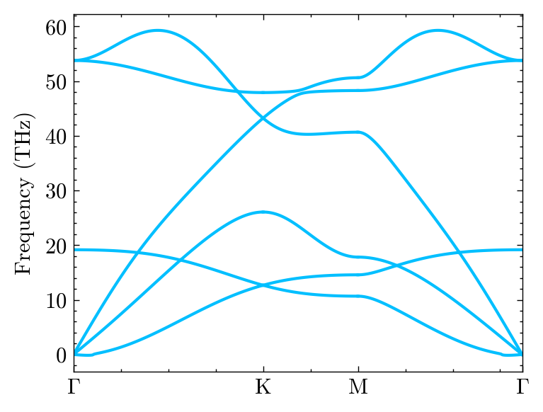
Then one can plot the band stucture.

fig, ax, _ = system.Phon.plot_dispersion()

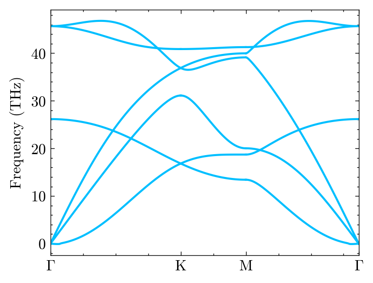
One can custom the figure detail.

# all parameters can be found in plt.rcParams
mp.pltset(**{"xtick.major.width":1.,
             "ytick.major.width":1.,
             "axes.linewidth":1.,
             'xtick.minor.visible':False,
             'ytick.minor.visible':False,
             })
fig, ax = mp.set_figure(figsize=(8, 8), figdpi=150)
fig, ax, _ = system.Phon.plot_dispersion(fig, ax, c='green', linestyle='-.')
ax.set_ylim(0, 50)

(0.0, 50.0)

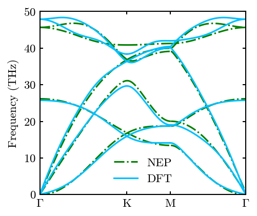
We can compare it with the DFT results. Note that, for scientific publication, one need to fully relax the cell before calculating phonon dispersion.

fig, ax = mp.set_figure(figsize=(8, 8), figdpi=150)
fig, ax, line1 = system.Phon.plot_dispersion(fig, ax, c='green', linestyle='-.')

fig, ax, line2 = system.Phon.plot_dispersion(fig, ax, filename='../../../example/gra.dat')

ax.legend([line1, line2], ['NEP', 'DFT'])
ax.set_ylim(0, 50)

(0.0, 50.0)

One can check the data.

system.Phon.bands_dict.keys()

dict_keys(['qpoints', 'distances', 'frequencies', 'eigenvectors', 'group_velocities'])

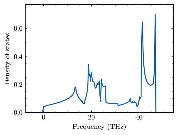
One can also compute the dos, pdos and thermal properties.

Computer dos

system.Phon.compute_dos(mesh=(30, 30, 30))

fig, ax = system.Phon.plot_dos()

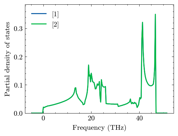
Compute pdos

system.Phon.compute_pdos(mesh=(30, 30, 30))

fig, ax = system.Phon.plot_pdos()

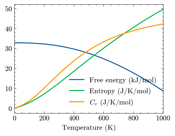
Compute thermal properties

system.Phon.compute_thermal(0, 50, 1000, mesh=(30, 30, 30))

fig, ax = system.Phon.plot_thermal()

Airebo potential

Here we show how to use a lammps potential to calculate the phonon. How to install lammps-python interface can be found in here. You can check it by: - from lammps import lammps

from mdapy.potential import LammpsPotential

One need to provide the pair_parameter in lammps format.

The airebo potential is downloaded from lammps example folder.

potential = LammpsPotential(
    """
    pair_style airebo 3.0
    pair_coeff * * ../../../example/CH.airebo C
    """
)

# Do computation
system.cal_phono_dispersion(path, labels, potential, elements_list=['C'])

Warning: Point group symmetries of supercell and primitivecell are different.

fig, ax, _ = system.Phon.plot_dispersion()

Some potential maybe need other setup and the units, such as reaxFF, we need to change the force units.

ReaxFF potential

This reaxff potential is downloaded from here.

potential = LammpsPotential(
    """
    pair_style      reax/c ../../../example/lmp_control
    pair_coeff      * * ../../../example/ffield.reax.GR-RDX-2021 Cg
    """,
    atomic_style='charge',
    units='real',
    extra_args='fix 1 all qeq/reax 1 0.0 10.0 1e-6 reax/c',
    conversion_factor={'energy':0, 'force':1/23.06, 'virial':0}
)

# here we do not care energy and virial, only need to converse force from
# kcal/mol/A to eV/A

# Do computation
system.cal_phono_dispersion(path, labels, potential, elements_list=['C'])

Warning: Point group symmetries of supercell and primitivecell are different.

fig, ax, _ = system.Phon.plot_dispersion()

Sometimes we want to use other potential not supported by lammps, we can define it for mdapy very easily. Here we use deepmd potential as an example.

User-defined potential

from mdapy.potential import BasePotential

One can install deepmd by:

• pip install deepmd-kit[cpu]

import deepmd

WARNING:tensorflow:From d:\Software\miniconda3\envs\mda\lib\site-packages\tensorflow\python\compat\v2_compat.py:108: disable_resource_variables (from tensorflow.python.ops.variable_scope) is deprecated and will be removed in a future version.
Instructions for updating:
non-resource variables are not supported in the long term

WARNING:root:To get the best performance, it is recommended to adjust the number of threads by setting the environment variables OMP_NUM_THREADS, TF_INTRA_OP_PARALLELISM_THREADS, and TF_INTER_OP_PARALLELISM_THREADS. See https://deepmd.rtfd.io/parallelism/ for more information.

deepmd.__version__

'2.2.10'

from deepmd.infer import DeepPot

class DP(BasePotential):

    def __init__(self, filename):
        self.filename = filename
        self.dp = DeepPot(self.filename)

    def compute(self, pos, box, elements_list, type_list, boundary=[1, 1, 1],):
        # This method must containe the above input parameter and keep the same order.
        # You can add other parameter if needed, and those parameter dose not need to be all used.
        # This method should return three parameters and the second is force array. The shape is (Natom, 3).
        # The units should be eV/A.

        coord = pos.reshape([1, -1])
        cell = box[:-1].reshape([1, -1])
        atype = type_list-1
        e, f, v = self.dp.eval(coord, cell, atype)
        return e, f[0], v

This deepmd potential downloaded from this paper. We convert it to new version:

• dp convert-from -i .:nbsphinx-math:carbon_16689_frozen_model_mmc1.pb -o carbon.pb

potential = DP("../../../example/carbon.pb")

WARNING:tensorflow:From d:\Software\miniconda3\envs\mda\lib\site-packages\deepmd\utils\batch_size.py:28: is_gpu_available (from tensorflow.python.framework.test_util) is deprecated and will be removed in a future version.
Instructions for updating:
Use `tf.config.list_physical_devices('GPU')` instead.

WARNING:tensorflow:From d:\Software\miniconda3\envs\mda\lib\site-packages\deepmd\utils\batch_size.py:28: is_gpu_available (from tensorflow.python.framework.test_util) is deprecated and will be removed in a future version.
Instructions for updating:
Use `tf.config.list_physical_devices('GPU')` instead.
WARNING:deepmd_utils.utils.batch_size:You can use the environment variable DP_INFER_BATCH_SIZE tocontrol the inference batch size (nframes * natoms). The default value is 1024.

# Do computation
system.cal_phono_dispersion(path, labels, potential, elements_list=['C'])

Warning: Point group symmetries of supercell and primitivecell are different.

fig, ax, _ = system.Phon.plot_dispersion()