QuicklyStart

This is a quick start guide to show users what mdapy can do and how it should be implemented, for more specific information check out the API in the documentation.

Import corresponding packages

[1]:

import mdapy as mp
import numpy as np
import os
mp.init() # Run on CPU

[Taichi] version 1.7.0, llvm 15.0.1, commit 2fd24490, win, python 3.8.0
[Taichi] Starting on arch=x64

[2]:

mp.__version__

[2]:

'0.10.7'

Generate a System class from a dump file, which can be found in example folder and come from the Supplementary materials of this paper.

[3]:

system = mp.System('../../../example/CoCuFeNiPd-4M.dump')

Check the data of System.

[4]:

system

[4]:

Filename: ../../../example/CoCuFeNiPd-4M.dump
Atom Number: 8788
Simulation Box:
[[47.36159615  0.          0.        ]
 [ 0.         47.46541884  0.        ]
 [ 0.          0.         47.46849764]
 [-1.18079807 -1.23270942 -1.23424882]]
TimeStep: 0
Boundary: [1, 1, 1]
Particle Information:
shape: (8_788, 5)
┌──────┬──────┬───────────┬───────────┬───────────┐
│ id   ┆ type ┆ x         ┆ y         ┆ z         │
│ ---  ┆ ---  ┆ ---       ┆ ---       ┆ ---       │
│ i64  ┆ i64  ┆ f64       ┆ f64       ┆ f64       │
╞══════╪══════╪═══════════╪═══════════╪═══════════╡
│ 1    ┆ 2    ┆ 0.006118  ┆ -0.310917 ┆ -0.345241 │
│ 2    ┆ 4    ┆ 1.9019    ┆ -0.292456 ┆ 1.48488   │
│ 3    ┆ 3    ┆ -0.015641 ┆ 1.58432   ┆ 1.43129   │
│ 4    ┆ 5    ┆ 1.86237   ┆ 1.51117   ┆ -0.372278 │
│ 5    ┆ 5    ┆ 3.79257   ┆ -0.331891 ┆ -0.37583  │
│ …    ┆ …    ┆ …         ┆ …         ┆ …         │
│ 8784 ┆ 3    ┆ 41.5595   ┆ 45.481    ┆ 43.4996   │
│ 8785 ┆ 4    ┆ 43.4575   ┆ 43.7371   ┆ 43.6083   │
│ 8786 ┆ 4    ┆ 45.3771   ┆ 43.7577   ┆ 45.2727   │
│ 8787 ┆ 4    ┆ 43.4552   ┆ 45.4854   ┆ 45.2825   │
│ 8788 ┆ 1    ┆ 45.3919   ┆ 45.4009   ┆ 43.4999   │
└──────┴──────┴───────────┴───────────┴───────────┘

[5]:

system.data.head()

[5]:

shape: (5, 5)

id	type	x	y	z
i64	i64	f64	f64	f64
1	2	0.006118	-0.310917	-0.345241
2	4	1.9019	-0.292456	1.48488
3	3	-0.015641	1.58432	1.43129
4	5	1.86237	1.51117	-0.372278
5	5	3.79257	-0.331891	-0.37583

Calculate the average entropy fingerprint.

[6]:

system.cal_atomic_entropy(rc=3.6*1.4, sigma=0.2, compute_average=True, average_rc=3.6*0.9)

Calculate the CSP.

[7]:

system.cal_centro_symmetry_parameter()

Calculate the CNA pattern.

[8]:

system.cal_common_neighbor_analysis(3.6*0.8536)

Calculate the Voronoi volume.

[9]:

system.cal_voronoi_volume()

Check the calculated results.

[10]:

system.data.head()

[10]:

shape: (5, 12)

id	type	x	y	z	atomic_entropy	ave_atomic_entropy	csp	cna	voronoi_volume	voronoi_number	cavity_radius
i64	i64	f64	f64	f64	f64	f64	f64	i32	f64	i32	f64
1	2	0.006118	-0.310917	-0.345241	-5.997978	-6.469179	0.100697	1	12.68101	15	3.675684
2	4	1.9019	-0.292456	1.48488	-6.640982	-6.677862	0.139544	1	12.012947	14	3.581766
3	3	-0.015641	1.58432	1.43129	-6.821837	-6.666713	0.094929	1	12.197214	12	3.674408
4	5	1.86237	1.51117	-0.372278	-6.95832	-6.940526	0.072999	1	12.900968	15	3.713117
5	5	3.79257	-0.331891	-0.37583	-6.679066	-6.846047	0.046358	1	12.400861	14	3.645415

Check the cutoff distance now.

[11]:

system.rc

[11]:

5.04

Neighbor atom index of atom 0 withing the cutoff distance.

[12]:

system.verlet_list[0][system.verlet_list[0]>-1]

[12]:

array([ 896, 8678,  897, 1009,    2, 7777,    3,    1,  110,  109, 7779,
       7885, 7782, 7785, 7778, 8677, 7776, 1012, 1010, 8683, 1008, 1007,
        902,  901,  899, 8785, 8787,  895,  894,  115,  113,  111, 7887,
       7886,  108,   10,    9,    7,    6,    5,    4, 8676, 8786, 7890])

Corresponding distance from atom 0 to its neighbor atoms.

[13]:

system.distance_list[0][system.verlet_list[0]>-1]

[13]:

array([2.51207536, 2.57315662, 2.5790717 , 2.58034708, 2.59777966,
       2.60048908, 2.60123122, 2.63508509, 2.63799678, 2.64905374,
       2.72325745, 2.75477797, 4.61796981, 4.39168494, 4.7209429 ,
       4.56321863, 3.89905168, 4.59982446, 4.55429458, 4.32684229,
       4.31587082, 5.02071962, 4.39625619, 4.94515597, 4.54722966,
       4.35032952, 4.48415811, 4.33703624, 3.40006539, 4.52692729,
       4.59187952, 4.58003206, 4.66009997, 4.7530261 , 3.73204146,
       4.42655427, 3.47691914, 4.43249288, 3.67048701, 4.59684361,
       3.78663373, 4.28528331, 4.63487348, 4.59095292])

Validate the distance between atom 0 and atom 896.

[14]:

system.atom_distance(0, 896)

[14]:

2.5120753608164965

Save the results to the disk.

[15]:

system.write_dump()

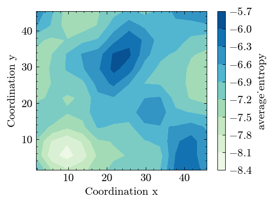
Do the spatial binning of entropy along xy plane.

[16]:

system.spatial_binning('xy', 'ave_atomic_entropy', 4.)

Binning coordinations.

[17]:

system.Binning.coor

[17]:

{'x': array([ 1.709397,  5.709397,  9.709397, 13.709397, 17.709397, 21.709397,
        25.709397, 29.709397, 33.709397, 37.709397, 41.709397, 45.709397]),
 'y': array([ 1.439891,  5.439891,  9.439891, 13.439891, 17.439891, 21.439891,
        25.439891, 29.439891, 33.439891, 37.439891, 41.439891, 45.439891])}

Plot the binning results.

[18]:

fig, ax = system.Binning.plot(value_label='average_entropy')

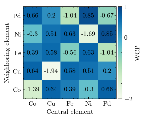
../_images/gettingstarted_quicklystart_35_0.png

Calculate the WCP to reveal the short-range order in alloy.

[19]:

system.cal_warren_cowley_parameter()

Results show high SRO degree.

[20]:

fig, ax = system.WarrenCowleyParameter.plot(['Co', 'Cu', 'Fe', 'Ni', 'Pd'])

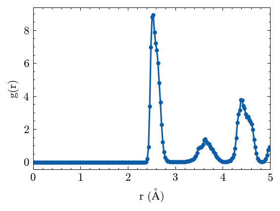
../_images/gettingstarted_quicklystart_39_0.png

Calculate the radiul distribution function (RDF).

[21]:

system.cal_pair_distribution()

Plot the RDF results.

[22]:

fig, ax = system.PairDistribution.plot()

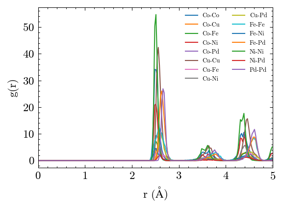
../_images/gettingstarted_quicklystart_43_0.png

Plot the partial RDF results.

[23]:

fig, ax = system.PairDistribution.plot_partial(['Co', 'Cu', 'Fe', 'Ni', 'Pd'])

../_images/gettingstarted_quicklystart_45_0.png

One can save the figure easily.

[24]:

fig.savefig('rdf.png', dpi=300)
os.remove('rdf.png') # Here just remove the saved figure.

Analyze the atomic trajectories

Generate a random walk trajectories.

[25]:

Nframe, Nparticles = 200, 1000
pos_list = np.cumsum(
    np.random.choice([-1.0, 1.0], size=(Nframe, Nparticles, 3)), axis=0
)*np.sqrt(2)

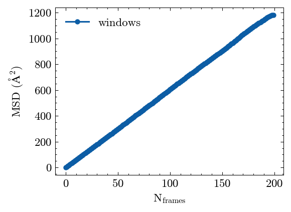
Calculate the mean squared displacement (MSD).

[26]:

MSD = mp.MeanSquaredDisplacement(pos_list=pos_list, mode="windows")
MSD.compute()

Check the MSD results.

[27]:

MSD.msd[:10]

[27]:

array([-1.91164418e-13,  6.00000000e+00,  1.19898990e+01,  1.79689746e+01,
        2.39582857e+01,  2.99463385e+01,  3.59534433e+01,  4.19486010e+01,
        4.79263750e+01,  5.38981361e+01])

Plot the MSD results.

[28]:

fig, ax = MSD.plot()

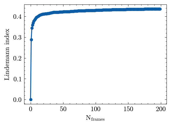
../_images/gettingstarted_quicklystart_56_0.png

Calculate the Lindemann index.

[29]:

LDML = mp.LindemannParameter(pos_list)
LDML.compute()

Plot the Lindemann index results.

[30]:

fig, ax = LDML.plot()

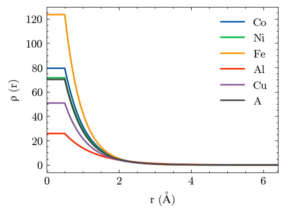
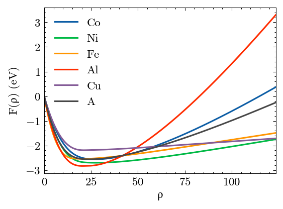
../_images/gettingstarted_quicklystart_60_0.png

Analyze EAM potential.

Generate an average EAM potential is simple.

[31]:

EAMave = mp.EAMAverage('../../../example/CoNiFeAlCu.eam.alloy', [0.2]*5)

Read this average potential file.

[32]:

potential = mp.EAM('./CoNiFeAlCu.average.eam.alloy')

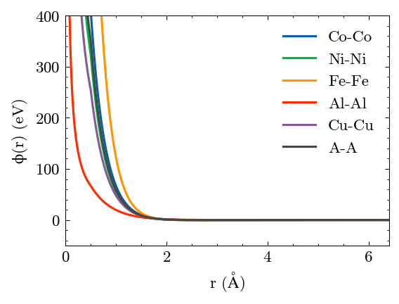
Plot the results. A is the virtual element.

[33]:

potential.plot()

../_images/gettingstarted_quicklystart_67_0.png

../_images/gettingstarted_quicklystart_67_1.png

../_images/gettingstarted_quicklystart_67_2.png

[34]:

os.remove('CoNiFeAlCu.average.eam.alloy') # Here just remove this average EAM file.